Approximating infinite series

In this post, I’ll derive the Euler-Maclaurin summation formula, which allows you to closely approximate a summation over a function $f$ by its integral.

For infinite series that are hard to evaluate analytically, we can sometimes resort to numeric evaluation, that is, we find a close approximation of the series.

For example, Euler famously applied this to the Basel problem, which asks for the value of ${\sum }_{k=1}^{\infty }\frac{1}{k^2}$. Before finding the analytical value $\frac{p{i}^2}{6}$, Euler found that $$\sum _{k=1}^{\infty }\frac{1}{k^2}\approx \mathrm{1.64493406...}$$

Euler found the first 20 fractional digits of the expression, and it is commonly believed that this convinced him that ${\sum }_{k=1}^{\infty }=\frac{{\pi }^2}{6}$, which he subsequently proved.

In this post, I’ll explain how Euler was able to find such an accurate approximation. We’ll start with a naive approximation method and figure out more accurate methods step-by-step.

Infinite sums, the naive way

Suppose we want to numerically evaluate ${\sum }_{k=1}^{\infty }f(k)$. In order for this sum to converge, $f$ must be a function that satisfies ${\lim }_{k\to \infty }f(k)=0$. By definition, we have $$\sum _{k=1}^{\infty }f(k)=\underset{N\to \infty }{\lim }\sum _{k=1}^{N}f(k)$$

So, as a first approximation to ${\sum }_{k=1}^{\infty }f(k)$, we can take some $N$ and evaluate the partial sum of the first $N$ terms. We expect the approximation to get better as $N$ gets larger.

This gives us our first, naive way of approximation ${\sum }_{k=1}^{\infty }f(k)$: For large $N$, we have $$\sum _{k=1}^{\infty }f(k)\approx \sum _{k=1}^{N}f(k)\text{\hspace{1em}(1)}$$

How well this method works depends greatly on how fast $f$ goes to 0.

TODO: examples here

Estimating the tail

We can write split the series explicitly in the partial sum of the first $N$ terms, and the other terms:

$$\sum _{k=1}^{N}f(k)=\sum _{k=1}^{N}f(k)+\sum _{k=N+1}^{\infty }f(k)\text{\hspace{1em}(2)}$$

By approximating an infinite series with a partial sum, we essentially drop the infinite “tail” ${\sum }_{k=N+1}^{\infty }f(k)$. Evaluating this sum directly is as hard as evaluating the original (complete) sum, but we can improve the accuracy of our initial approximation by adding an approximation to the infinite sum.

For this, we can use the approximation

$$\sum _{k=a}^{b-1}f(k)\approx {\int }_a^{b}f(x)\text{d}x$$

This gives us an improved formula for approximating ${\sum }_{k=1}^{N}f(k)$: $$\sum _{k=1}^{\infty }f(k)\approx \sum _{k=1}^{N}f(k)+{\int }_{N+1}^{\infty }f(x)\text{d}x\text{\hspace{1em}(3)}$$

TODO: examples

A geometric improvement

Now, again, we want to improve the accuracy of the approximation $$\sum _{k=a}^{b-1}f(k)\approx {\int }_a^{b}f(x)\text{d}x$$

Using ${\sum }_{k=a}^{b-1}f(k)={\int }_a^{b}f(\lfloor x\rfloor )\text{d}x$ we can write the error $E(x)$ explicitly as $E(x)=f(\lfloor x\rfloor )-f(x)$. We now have $$\sum _{k=a}^{b-1}f(k)={\int }_a^{b}f(x)+E(x)\text{d}x\text{\hspace{1em}(4)}$$

Let’s visualize this and draw $f(x)$, $f(\lfloor x\rfloor )$, and $E(x)$ in a single graph:

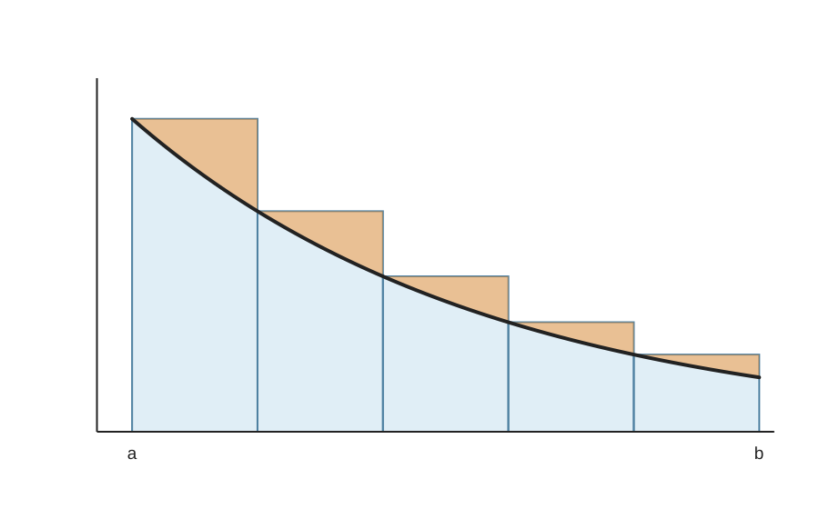
Gathering the shaded segments on the left, we can see that the shaded areas look a lot like triangles:

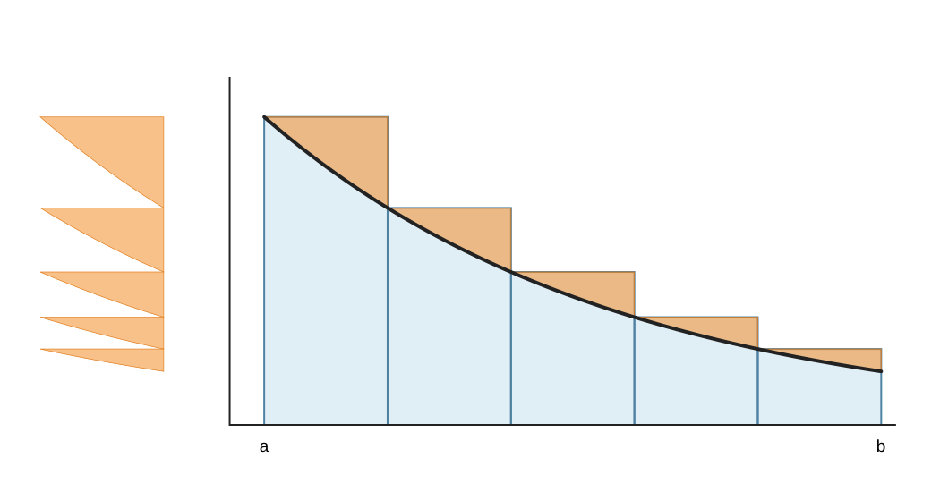
We can therefore estimate the shaded area on the interval $[k,k+1]$ with the formula for the area of a triangle: $${\int }_k^{k+1}E(x)\text{d}x\approx \frac{f(k)-f(k+1)}{2}$$

If we plug this into $(4)$, we get $$\sum _{k=a}^{b-1}f(k)\approx {\int }_a^{b}f(x)\text{d}x+\frac{f(a)-f(b)}{2}\text{\hspace{1em}(5)}$$

Setting $a=N+1$, $b=\infty$ and using that ${\lim }_{k\to \infty }f(k)=0$ gives us $$\sum _{N+1}^{\infty }f(k)\approx {\int }_{N+1}^{\infty }f(x)\text{d}x+\frac{f(N+1)}{2}$$

If we plug this into $(2)$, we get $$\sum _{k=1}^{\infty }f(k)\approx \sum _{k=1}^{N}f(k)+{\int }_{N+1}^{\infty }f(x)\text{d}x+\frac{f(N+1)}{2}\text{\hspace{1em}(6)}$$

This is again an improvement over the previous approximation formula.

TODO: examples

A natural question is now if we can further improve this method. Intuitively you’d expect a connection with the first derivative of $f$, and it feels like you might be able to generalize this to higher-order derivatives. However, geometrically it’s not clear exactly how this would generalize.

Analysis with Taylor series

Let’s try to see what’s going on through the lens of Taylor series.

If we take $(5)$ and set $a=k$, $b=k+1$, the summation is just over a single term. Using ${\int }_k^{k+1}f(x)\text{d}x={\int }_0^{1}f(k+t)\text{d}t$ we get $$f(k)={\int }_0^{1}f(k+t)\text{d}t+\frac{f(k)-f(k+1)}{2}\text{\hspace{1em}(7)}$$

Using the Taylor expansion of $f(x)$ at $x=k$, we get $$f(k+t)=f(k)+f^{\prime }(k)t+\frac{f^{\prime \prime }(k)}{2}{t}^2+...$$

We can substitute the Taylor series both in ${\int }_0^{1}f(k+t)\text{d}t$ and $f(k+1)$: $$\begin{array}{rl}{\int }_0^{1}f(k+t)\text{d}t& =f(k)+\frac{f^{\prime }(k)}{2}+\frac{f^{\prime \prime }(k)}{6}+...\\ f(k+1)& =f(k)+f^{\prime }(k)+\frac{f^{\prime \prime }(k)}{2}+...\end{array}$$

Substituting these expressions back in $(7)$ gives $$\begin{gathered} {\int }_0^{1}f(k+t)\text{d}t+\frac{f(k)-f(k+1)}{2} \\ =f(k)-\frac{1}{12}{f}^{\prime \prime }(k)+... \end{gathered}$$

In other words, the term $\frac{f(k)-f(k+1)}{2}$ serves as a correction that cancels the term involving $f^{\prime }(k)$ in the Taylor expansion of ${\int }_0^{1}f(k+t)\text{d}t$. The rest terms now only derivatives of at least second order. For smooth functions we expect that the magnitude of higher derivatives is much smaller than that of lower derivatives, which explains why $(6)$ is a better approximation to $f(k)$ than $(3)$.

General case

In the previous section we saw that adding the term $\frac{f(k)-f(k+1)}{2}$ cancels the terms involving first order derivatives in the Taylor expansion of ${\int }_0^{1}f(k+t)\text{d}t$. This idea generalizes in a straightforward way: We’ll now try to cancel the terms involving the first $N$ derivatives.

That is, we try to find $c_0$, $c_1$, …, $c_{N-1}$ such that $${\int }_0^{1}f(k+t)\text{d}t+\sum _{i=0}^{N-1}{c}_i(f^{(i)}(k)-f^{(i)}(k+1))$$

contains no terms involving $f^{\prime }(k)$, $f^{\prime \prime }(k)$, …, $f^{(N)}(k)$. This happens exactly when the coefficients of $f^{(n)}(k)$ in the Taylor expansions of ${\int }_0^{1}f(k+t)\text{d}t$ and $-{\sum }_{i=0}^{N-1}{c}_i(f^{(i)}(k)-f^{(i)}(k+1))$ match for $n=1,2,...,N$.

Using the Taylor expansion of $f(x)$ at $x=k$ we get $${\int }_0^{1}f(k+t)\text{d}t=\sum _{j=0}^{\infty }\frac{1}{(j+1)!}{f}^{(j)}(k)$$

So the coefficient of $f^{(n)}$ in the Taylor expansion of ${\int }_0^{1}f(k+t)\text{d}t$ is $\frac{1}{(n+1)!}$.

Likewise we have $-{\sum }_{i=0}^{N-1}{c}_j(f^{(j)}(k)-f^{(j)}(k+1))={\sum }_{i=0}^{N-1}{c}_j(f^{(j)}(k+1)-f^{(j)}(k))$ and

$$c_i(f^{(i)}(k+1)-f^{(i)}(k))=\sum _{j=1}^{\infty }\frac{c_i}{j!}{f}^{(i+j)}(k)$$

So the coefficient of $f^{(n)}$ in the Taylor expansion of $-{\sum }_{i=0}^{N-1}{c}_j(f^{(j)}(k)-f^{(j)}(k+1))$ is ${\sum }_{i=0}^{n-1}\frac{c_i}{(n-i)!}$.

Equating the two gives $$\sum _{i=0}^{n-1}\frac{1}{(n-i)!}{c}_i=\frac{1}{(n+1)!}\text{\hspace{1em}(8)}$$

Evaluating this relation for $n=1$ gives $c_0=\frac{1}{2}$. For $n=2$ it gives $$\frac{1}{2!}{c}_0+\frac{1}{1!}{c}_1=\frac{1}{3!}$$

Substituting $c_0=\frac{1}{2}$ gives $c_1=-\frac{1}{12}$. Now, we can set $n=3$ and substitute the values for $c_0$ and $c_1$ to find $c_2$. We can continue this strategy to compute all the coefficients we need.

The first 10 coefficients are: $$\frac{1}{2},-\frac{1}{12},0,\frac{1}{720},0,-\frac{1}{30240},0,-\frac{1}{1209600},0,-\frac{1}{47900160}$$

Demonstration

Relation to the Bernoulli numbers

Taking $(8)$ and multiplying it by $(n+1)!$ we get $$\sum _{i=0}^{n-1}\frac{(n+1)!}{(n-i)!}{c}_i=1$$

We have $\frac{(n+1)!}{(n-i)!}=\left(\genfrac{}{}{0ex}{}{n+1}{i+1}\right)\cdot (i+1)!$, so let’s substitute $c_i=(i+1)!B_{i+1}$ so we can simplify. We get $$\sum _{i=1}^n\left(\genfrac{}{}{0ex}{}{n+1}{i}\right)B_i=1$$

This is a recurrence relation for the Bernoulli numbers $B_1$, $B_2$, … However, the recurrence relation doesn’t account for the first Bernoulli number $B_0$. If we boldly extend the summation to $i=0$ and set $n=0$ we get $\left(\genfrac{}{}{0ex}{}{1}{0}\right)B_0=1$, which is indeed correct. For $n>0$ we have $$\sum _{i=0}^n\left(\genfrac{}{}{0ex}{}{n+1}{i}\right)B_i=1+\sum _{i=1}^n\left(\genfrac{}{}{0ex}{}{n+1}{i}\right)B_i$$

So we have found the following recurrence relation for the Bernoulli numbers: $$\sum _{i=0}^n\left(\genfrac{}{}{0ex}{}{n+1}{i}\right)B_i={\delta }_{n,0}$$

Here, ${\delta }_{n,0}$ is defined as $${\delta }_{n,0}=\{\begin{array}{l}1\text{when n=0}\\ 0\text{when n=0}\end{array}$$