B-splines

This is an edited section from my thesis “Solving Poisson’s equation with Dataflow computing”. It might be a bit more formal than most of my other posts.

Splines are a mathematical concept which can be used to define smooth (or less smooth) curves and surfaces.

In this article, I’ll cover some mathematical background.

Introduction to splines

Splines (or spline functions) are also called piecewise polynomial. The reason is illustrated by the following definition:

Definition: A spline or piecewise polynomial function of degree $p$ is a function $f:\mathbb{R}\to \mathbb{R}$, such that there exist ${\xi }_0<{\xi }_1<...<{\xi }_m$ and polynomials $p_0$, $p_1$, …, $p_{m-1}$ with degree at most $p$ such that $f(x)=p_k(x)$ if $x\in ({\xi }_k,{\xi }_{k+1})$, and either $f(x)=p_k(x)$ or $f(x)=p_{k+1}(x)$ when $x={\xi }_{k+1}$. The values ${\xi }_0$, ${\xi }_1$, …, ${\xi }_m$ are called breaks.

In order to define spline spaces, we introduce the concept of a knot vector:

Definition: A knot vector $\mathbf{\Xi }$ is a non-decreasing vector $({\xi }_0,{\xi }_1,...,{\xi }_m)$. The values ${\xi }_0$, ${\xi }_1$, …, ${\xi }_m$ are called knots, and the number of times that a knot ${\xi }_k$ occurs in the knot vector is called the multiplicity ${\mu }_k$ of the knot.

We can now define a space of splines, where the continuity along the breaks is defined by the multiplicities of the knots:

Definition: The spline space ${\mathbb{S}}_p(\mathbf{\Xi })$ of degree $p$ for a knot vector $\mathbf{\Xi }=({\xi }_0,{\xi }_1,...,{\xi }_m)$ is defined as the space of splines $s$ of order $p$, with breaks ${\xi }_0$, ${\xi }_1$, …, ${\xi }_m$ and support on a subset of $[{\xi }_0,{\xi }_m]$. Furthermore, we require that $s$ is $C^{p-{\mu }_k}$-continuous on ${\xi }_k$, for $k=0$, $1$, …, $m$.

To ensure that ${\mathbb{S}}_p(\mathbf{\Xi })$ is well-defined and continuous, we demand that $\mathbf{\Xi }$ is a knot vector of degree $p$.

Definition: A knot vector is called a knot vector of degree $p$ if all knots have a multiplicity of at most $p$.

It should be noted that the requirement that $s$ is continuous implies that $s({\xi }_0)=0$ and $s({\xi }_m)=0$. Sometimes, this is not desirable. To remove this restriction, the concept of an open knot vector of degree $p$ is introduced:

Definition: A knot vector is called an open knot vector of degree $p$ when the first and last knot have multiplicity $p+1$, and all other knots have a multiplicity of at most $p$.

It should be noted that, according to these definitions, an open knot vector of degree $p$ is not a knot vector of degree $p$. We will work with knot vectors with uniformly distributed knots on the interval $[0,1]$.

Definition: A knot vector $\mathbf{\Xi }=({\xi }_0,{\xi }_1,...,{\xi }_m)$ is called a uniform knot vector when ${\xi }_k-{\xi }_{k-1}=c$ for all $k=1,2,...,m$ and some constant $c>0$. A knot vector of the same form is called a uniform open knot vector of degree $p$ when ${\xi }_0$ and ${\xi }_n$ have multiplicity $p+1$, and ${\xi }_{k+1}-{\xi }_k=c$ for $k=p+1,p+2,...,m-p$ and some constant $c>0$.

B-splines

The term ‘B-spline’ is an abbreviation for ‘basis spline’. B-splines were introduced as basis functions for the spline space. However, the CAD community has adopted the term to refer to splines which are represented in terms of these basis functions. This has caught on, and it has become common to call the basis functions ‘B-spline basis functions’. This is the terminology that will be used in this document as well.

The recursive definition that is commonly used to introduce B-splines was presented in [2] by de Boor.

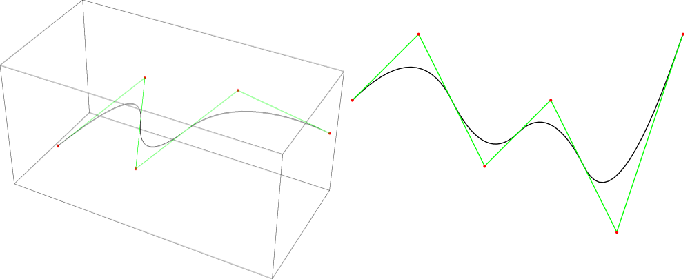
Definition: For $d\ge 1$, a $d$-dimensional B-spline curve $\mathbf{s}:\mathbb{R}\to {\mathbb{R}}^d$ is defined as a linear combination of B-spline basis functions $N_{0,p},N_{1,p},...,N_{n-1,p}:\mathbb{R}\to \mathbb{R}$:

The image $\mathbf{s}$ is a one-dimensional subset of ${\mathbb{R}}^d$. It is common to identify $\mathbf{s}$ with this subset and refer to both as a B-spline curve. The coefficients ${\mathbf{c}}_0,{\mathbf{c}}_1,...,{\mathbf{c}}_{n-1}\in {\mathbb{R}}^d$ are called control points, and the B-spline basis functions $N_{0,p},N_{1,p},...,N_{n-1,p}:\mathbb{R}\to \mathbb{R}$ are defined by the Cox-de-Boor recursion formula. The following version is from [3]:

where

$p$ is called the polynomial degree, and $\mathbf{\Xi }=({\xi }_0,{\xi }_1,...,{\xi }_{n+p})$ is a knot vector of degree $p$

The index $p$, denoting the polynomial degree, will often be omitted when its value is irrelevant or clear from the context, so that $N_i$ denotes the same basis function as $N_{i,p}$.

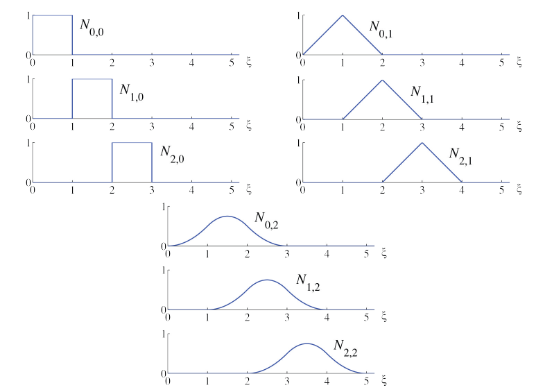
The next image shows the B-spline basis functions associated to the uniform knot vector $\mathbf{\Xi }=(0,\frac{1}{6},\frac{1}{3},\frac{1}{2},\frac{2}{3},\frac{5}{6},1)$ for polynomials orders $p=0,1,2,3$:

The following characterization of B-spline basis functions is due to Curry and Schoenberg in [4] and [5]:

Theorem (Curry-Schoenberg): The set of B-spline basis functions $N_{p,0},N_{p,1},...,N_{p,n}:\mathbb{R}\to \mathbb{R}$ associated to the knot vector $\mathbf{\Xi }=({\xi }_0,{\xi }_1,...,{\xi }_{n+p})$ is a basis for the spline space ${\mathbb{S}}_p(\mathbf{\Xi })$. Moreover, the B-splines basis functions have minimal support: for any $f\in {\mathbb{S}}_p(\mathbf{\Xi })$ with $f\ne 0$ we have that there exists a basis function $N_k$ with $\text{supp}(N_k)\subseteq \text{supp}(f)$.

For a proof that $N_{p,0},N_{p,1},...,N_{p,n}$ is a basis of ${\mathbb{S}}_p(\mathbf{\Xi })$, see [6], chapter 1, theorem 1.8 on page 8, or [4]. For a proof that the B-spline basis functions have minimal support, see [5].

In computer-aided design (CAD), it is convenient to have continuous curves that interpolate the first and last control point. This means that $\mathbf{s}(0)={\mathbf{c}}_0$, and $\mathbf{s}(1)={\mathbf{c}}_{\mathbf{n}-1}$ if ${\mathbf{c}}_{\mathbf{n}-1}$ is the last control point. This can be achieved by using an open knot vector to define the B-spline basis functions. The effect of taking the open knot vector $\mathbf{\Xi }=(0,0,0,\frac{1}{5},\frac{2}{5},\frac{3}{5},\frac{4}{5},1,1,1)$ of degree 2 is illustrated in the next image.

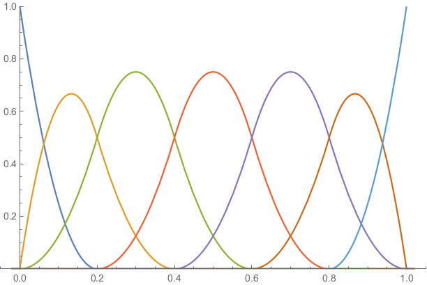
It can be seen that the first and the last B-spline basis functions $N_0$ and $N_6$ are discontinuous at the first knot ${\xi }_0=0$, and the last knot ${\xi }_7=1$, since $N_0(\xi )=0$ for $\xi <0$, but $N_0(0)=1$. Likewise, we have ${\lim }_{\xi \to 1}{N}_6\xi =1$, but $N_6(\xi )=0$ for $\xi \ge 1$. However, since $\mathbf{s}$ is only defined on $[0,1)$, $\mathbf{s}$ is still continuous. In practice, we will extend the domain of $\mathbf{s}$ to $[0,1]$ by the following convention.

Convention: Unless indicated otherwise, the knot vector $\mathbf{\Xi }=({\xi }_0,{\xi }_1,...,{\xi }_{n+p})$ used to define B-spline basis functions of degree $p$, is an open knot vector that satisfies ${\xi }_p=0$, ${\xi }_n=1$. Moreover, the domain of B-spline curves will be taken as $[0,1]$, with the convention

This convention ensures that B-spline curves are continuous mappings from $[0,1]$ to ${\mathbb{R}}^d$. In code, this is achieved by including a special check for the last basis function: If the last basis function is evaluated at the last knot of an open knot vector, it should evaluate to one (instead of zero).

Theorem: Suppose that $\mathbf{\Xi }=({\xi }_0,{\xi }_1,...,{\xi }_{n+p})$ is a (not necessarily open) knot vector of degree $p$. Then the basis functions $N_0,N_1,...,N_{n-1}$ of order $p$ associated to $\mathbf{\Xi }$, and the B-spline curve $\mathbf{s}$ as defined in $(1)$ satisfy the following properties:

1. $N_{0,p}$, $N_{1,p}$, …, $N_{n-1,p}\in {\mathbb{S}}_p(\mathbf{\Xi })$
2. If the derivative of a B-spline basis function $N_{i,p}$ exists at a point $\xi$, it is given by

3. The B-spline basis functions satisfy ${\sum }_{i=0}^{n-1}{N}_i=1$ and ${\sum }_{i=0}^{n-1}{N}_i^{\prime }=0$.
4. For a B-spline basis function $N_{i,p}$ we have $\overline{\text{supp}(N_{i,p})}=\overline{\text{supp}(N_{i,p}^{\prime })}=[{\xi }_i,{\xi }_{i+p+1}]$. Moreover ${\xi }_i\in \text{supp}(N_{i,p})$ iff $p=0$ or $i=0$ and $\mathbf{\Xi }$ is an open knot vector of degree $p$.
5. $\int N_{i,p}(\xi )N_{j,p}(\xi )\text{d}\xi$, $\int N_{i,p}(\xi )N_{j,p}^{\prime }(\xi )\text{d}\xi$, $\int N_{i,p}(\xi )N_{j,p}^{\prime }(\xi )\text{d}\xi$, and $\int N_{i,p}^{\prime }(\xi )N_{j,p}^{\prime }(\xi )\text{d}\xi$ are all zero whenever $|i-j|>p$. It follows that

6. The B-spline basis functions satisfy $0\le N_{i,p}\le 1$ and $-\frac{p}{h}\le N_{i,p}^{\prime }\le \frac{p}{h}$, where $h:={\min }_{i\in \{1,2,...,n\}}\{{\xi }_i-{\xi }_{i-1}:{\xi }_{i-1}\ne {\xi }_i\}$ is the smallest nonzero difference between two consecutive knots.
7. On any point in the $\mathbb{R}$, there are at most $p+1$ nonzero basis functions. More specifically, there are $p+1$ nonzero basis functions on $\xi \in ({\xi }_p,{\xi }_n)$, whenever $\xi \notin \mathbf{\Xi }$ is not a knot.
8. If $\mathbf{\Xi }$ is an open knot vector, $\mathbf{s}$ interpolates the first and last control points: $\mathbf{s}(0)={\mathbf{c}}_0$, $\mathbf{s}(1)={\mathbf{c}}_{n-1}$.

Proof: A sketch of the proofs is given. The interested reader can try to prove the properties more rigorously, or look at proofs given in [2], [6] or [7]. The first property follows from the Curry-Schoenberg theorem. The second property can be proved by taking the derivative of the recursive definition of the B-spline basis functions. Using the definition of a B-spline basis function, it can be proved by induction on the degree $p$ that ${\sum }_{i=0}^{n-1}{N}_{i,p}(\xi )=1$ should be treated differently, since the value is defined by the convention that is introduced). By taking the derivative of both sides, it follows that ${\sum }_{i=0}^{n-1}{N}_{i,p}^{\prime }=0$, and the third property follows. The fourth property follows from the definition of the B-spline basis functions by induction (except for the case $i=n-1$, which follows from the convention we use). The fifth property follows from the fourth. The sixth property follows from the second and third property. The seventh property follows from the fourth. For the eighth property, we can prove that $N_{p-j,j}(0)=1$ for $0\le j\le p$ by using the definition of the B-spline basis functions and induction on $j$. Likewise we have $N_{n-1,p}(1)=1$ by the used convention. From the third property we have ${\sum }_{i=0}^{n-1}{N}_i=1$, so that it follows that $\mathbf{s}(0)={\mathbf{c}}_0$, $\mathbf{s}(1)={\mathbf{c}}_{n-1}$.
$\square$

Now, the problem of finding an interpolating B-spline is considered. Suppose that we define a one-dimensional B-spline $f(\xi )=\sum _{j=0}^{n-1}{f}_j{N}_j(\xi )$ and we want to choose the control points $f_0$, $f_1$, …, $f_{n-1}$ such that $f({\xi }_0)=y_0$, $f({\xi }_1)=y_1$, …, $f({\xi }_{m-1})=y_{m-1}$. This is called the interpolation problem. We have the following theorem:

Theorem (Whitney-Schoenberg): For basis functions $N_{i_0}$, $N_{i_1}$, …, $N_{i_{n-1}}$ with $i_0<i_1<...<i_{n-1}$ which are a subset of the B-spline basis functions $N_0$, $N_1$, … associated to a not necessarily open knot vector $\mathbf{\Xi }$, and interpolations points ${\xi }_0<{\xi }_1<...<{\xi }_{m-1}$, the interpolation matrix $\mathbf{J}$ is nonsingular if and only if $n=m$, and

See [6], section 3.3, theorem 3.2 on page 19 for a proof.

Given a knot vector, it is not immediately obvious how we can choose interpolation points that satisfy the conditions of the Whitney-Schoenberg theorem. For this purpose, one can define the Greville abscissae:

Definition: For a knot vector $\mathbf{\Xi }=({\xi }_0,{\xi }_1,...,{\xi }_{m-1})$ of degree $p$, the Greville abscissae $x_0,x_1,...,x_{m-p-1}$ are defined as

Theorem: For B-spline basis functions $N_{0,p},N_{1,p},...,N_{n-1,p}$ associated to an open knot vector $\mathbf{\Xi }=({\xi }_0,{\xi }_1,...,{\xi }_{n+p})$ of degree $p$ we have

Proof: Suppose that ${\xi }_k=x_k$. Then we have ${\xi }_k={\xi }_{k+1}=...={\xi }_{k+p}$. So, the knot ${\xi }_k$ has multiplicity $p+1$.

If $k\ne 0,n-1$, we have that the multiplicity of ${\xi }_{k+1}$ is at most $p$. So, we can’t have ${\xi }_k={\xi }_{k+1}=...={\xi }_{k+p}$ or ${\xi }_{k+1}={\xi }_{k+2}=...={\xi }_{k+p+1}$ and both inequalities are strict, so we have $x_k\in ({\xi }_k,{\xi }_{k+p+1})$. By property 4, it follows that $N_k(x_k)\ne 0$.

If $k=0$, then${\xi }_k$ is the first knot, and has multiplicity $p+1$, so it follows that ${\xi }_k={\xi }_{k+1}=...={\xi }_{k+p}=0<{\xi }_{p+1}$. So it follows that $x_k=0$, and we have $N_0(0)=1$ by property 4.
$\square$

This means that the Greville abscissae are suitable as a standard choice for interpolation points for B-splines.

References

[1] C. De Boor. Splines as Linear Combinations of B-splines. A Survey.

[2] Carl de Boor. On calculating with B-splines.

[3] Carl de Boor. B(asic)-Spline Basics.

[4] H. B. Curry and Schoenberg I. J. On spline distributions and their limits: The Pólya distribution functions.

[5] H. B. Curry and Schoenberg I. J. On Pólya frequency functions IV: The fundamental spline functions and their limits.

[6] Tomas Sauer. Splines in Industrial Applications.

[7] Les Piegl and Wayne Tiller. The NURBS Book.